2611.00121v1 · First listed 2026-11-03
Beyond Point Photo-$z$ Estimates: Normalizing Flows for Tomographic $N(z)$ Reconstruction with DESI DR1
On a spatially independent DESI DR1 test set, conditional normalizing-flow redshift PDFs generally reconstruct tomographic N(z) better than quantile random forests, especially at high redshift; calibration improves several low-z mean-redshift biases but leaves population-transfer and residual-calibration limitations. [1][4][5]
Evidence
The authors train conditional normalizing flows (NFs) on about 1.1 million DESI DR1 galaxy and quasar targets with Legacy Surveys DR10 photometry, then evaluate five independent NF realisations on 2,028,371 objects in a non-overlapping sky region spanning roughly 0<z_spec<4.5. They compare NF posterior PDFs and their medians with RF and QRF models using point-photo-z metrics and stacked-PDF N(z) metrics, including Wasserstein distance, Jensen–Shannon divergence, overlap, and mean-redshift bias. At z_median>2.5, the abstract reports NF |Δz_mean|=0.060±0.031 and overlap 0.905±0.008, versus QRF values 0.318 and 0.787. The stated NF uncertainty reflects variation among realisations; no QRF uncertainty is given there. [1][3][4]
Earlier work
A supplied earlier DESI-based study calibrates tomographic n(z) for the HSC PDR3 shape catalogue and explicitly treats DESI DR1 ELG fibre-collision incompleteness. That is a distinct, clustering/calibration-oriented setting from this paper’s supervised photo-z PDF reconstruction, so the extracts do not support a direct numerical performance comparison. The current authors also state that their high-z point-estimation behavior is consistent with Ren et al. (2026), but that paper is not supplied here. [11][3]
What changes
The central extension is evaluation at the distribution level rather than only ranking point estimates: stacking continuous NF PDFs is tested in eight tomographic selections and against QRF stacking. The authors additionally derive redshift-dependent empirical-CDF recalibration mappings from a held-out validation region. After transfer to the independent test region, bins with 0.2<z_median<1 have absolute mean-redshift biases of 0.0016–0.0019, below the cited 0.002(1+z) Euclid benchmark in central value. [1][5]
Limits and open questions
Calibration makes test-set PIT distributions closer to uniform but leaves residual excesses, and improved probabilistic calibration does not improve every N(z) metric. All methods deteriorate above z_spec=1.6, where training data are limited. The reported high-z advantage is partly stress-tested with matched sample sizes (10,142 per model), but the selected NF and QRF populations need not be the same. The authors further flag run-to-run variability and uncertain generalisation to different photometric populations; thus these results do not by themselves establish performance for a weak-lensing source sample. [5][6][8][2]
The supplied extraction includes the abstract, conclusions, and selected appendices, but not full result tables or model-architecture passages. Figure assessments rely on the supplied caption list and corresponding conclusion extracts; detailed per-bin metrics beyond those explicitly quoted cannot be recovered.
Key figures
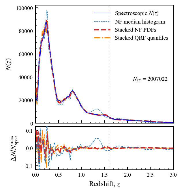
Tests whether stacking NF or QRF PDFs recovers the full spectroscopic N(z), rather than merely producing useful posterior-median point estimates; residuals are normalized by the peak of the reference distribution.
Original caption
Figure 3: Comparison of the reconstructed redshift distributions, N ( z ) N(z) , for the testing sample displayed over 0 < z < 3 0<z<3 for clarity. The upper panel shows the spectroscopic reference distribution alongside the reconstructions obtained by stacking the normalizing-flow (NF) and quantile random forest (QRF) PDFs, as well as the distribution of NF posterior-median redshift estimates. The lower panel shows the corresponding residuals relative to the spectroscopic distribution, normalised by its maximum value, Δ N / N spec max \Delta N/N_{\rm spec}^{\rm max} , where Δ N = N pred − N spec \Delta N=N_{\rm pred}-N_{\rm spec} . The vertical dotted line at z = 1.6 z=1.6 approximately separates the galaxy-dominated and quasar-dominated redshift ranges.
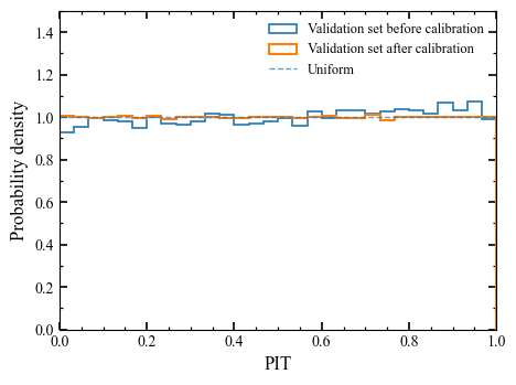
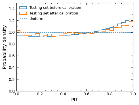
Tests transferability of validation-derived PDF recalibration: PIT histograms are compared before and after calibration in both validation and spatially independent testing samples.
Original caption
Figure 7: PIT distributions (30 bins) for the independent validation sample (upper panel) and testing sample (lower panel), shown before and after applying the calibration mapping derived from the validation set. The dashed horizontal line marks the ideal uniform distribution. After calibration, the validation-sample PIT is close to uniform, while the testing-sample PIT shows only modest improvement, with residual excesses remaining.
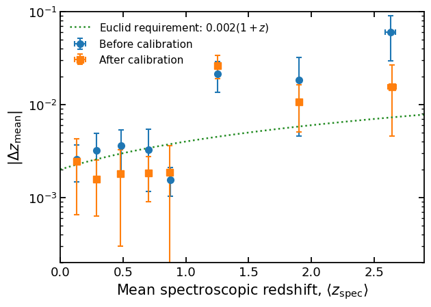
Tests tomographic mean-redshift accuracy before and after calibration across eight posterior-median bins. Points average independent NF realisations and error bars show their sample standard deviations against the Euclid benchmark.
Original caption
Figure 9: Absolute mean-redshift bias, | Δ z mean | = | ⟨ z pred ⟩ − ⟨ z spec ⟩ | |\Delta z_{\rm mean}|=|\langle z_{\rm pred}\rangle-\langle z_{\rm spec}\rangle| , as a function of the mean spectroscopic redshift for eight tomographic bins before (blue circles) and after (orange squares) post-hoc calibration. The points represent the mean absolute biases over independent NF realisations, with error bars indicating the sample standard deviations. The green dotted line indicates the Euclid mean-redshift accuracy benchmark, 0.002 ( 1 + z ) 0.002(1+z) . Tomographic bins are defined using the posterior-median redshift, z median z_{\rm median} , and galaxy membership is recomputed after calibration, accounting for the small differences in the mean spectroscopic redshifts before and after calibration. The lower error bar for the fifth tomographic bin extends below the plotted lower limit and is therefore partially truncated on the logarithmic y y -axis.
Related research
Previous digest
Chen et al. test conditional normalizing flows for probabilistic photometric-redshift inference and tomographic redshift-distribution reconstruction using DESI DR1 spectroscopy matched to Legacy Surveys DR10 photometry. Trained on 1.1 million DESI galaxy and quasar targets and evaluated on 2.0 million sources in a separate sky region, the flow produces better stacked N(z) reconstructions than quantile random forests, especially in the quasar-dominated high-redshift regime: at z_median > 2.5 it lowers the absolute mean-redshift bias from 0.318 to 0.060±0.031 and raises the distribution overlap from 0.787 to 0.905±0.008. A redshift-dependent post-hoc calibration brings the low-redshift tomographic-bin biases below the Euclid-style 0.002(1+z) benchmark and reduces the highest-bin bias to 0.016±0.011. The main limitation is transferability: results from DESI-selected spectroscopic targets may not carry directly to broader photometric populations with different selection functions.
Sources and evidence (26)
- 2611.00121v1: Beyond Point Photo-$z$ Estimates: Normalizing Flows for Tomographic $N(z)$ Reconstruction with DESI DR1
Accurate calibration of tomographic redshift distributions, $N(z)$ is essential for cosmological analysis of weak lensing data. We investigate conditional normalizing flows (NFs) and compare their performance with random forest (RF) and quantile random forest (QRF) models. We consider DESI galaxy and quasar targets from DESI DR1 spectroscopic data and with the photometry from Legacy Surveys DR10. We train on 1.1 million sources and test on 2.0 million sources in a non-overlapping sky region ($0<z_{\rm spec}<4.5$). For point estimation, the NF achieves the lowest scatter and outlier fraction at $0<z_{\rm spec}<1.6$ and outperforms both baselines across all three metrics at $z_{\rm spec}>1.6$. By introducing distribution-level metrics like Wasserstein distance and JS divergence, we find that stacking NF posterior PDFs provides more accurate tomographic $N(z)$ reconstruction than QRF, particularly at high redshifts. For $z_{\rm median}>2.5$, the NF achieves a smaller absolute mean-redshift bias ($0.060\pm0.031$ versus $0.318$) and higher probability overlap ($0.905\pm0.008$ versus $0.787$) than QRF. We apply redshift-dependent post-hoc PDF calibration derived from a held-out validation sample. After calibration, the absolute mean-redshift biases in four bins spanning $0.2<z_{\rm median}<1.0$ range from $0.0016$ to $0.0019$, with central values below referring benchmark $0.002(1+z)$. In the highest-redshift bin, calibration further reduces the bias to $0.016\pm0.011$. Our results demonstrate the potential of NF PDFs for tomographic $N(z)$ reconstruction while highlighting challenges in transferring models across galaxy populations.
- 2611.00121v1: Beyond Point Photo-$z$ Estimates: Normalizing Flows for Tomographic $N(z)$ Reconstruction with DESI DR1
The resulting tomographic redshift distributions are presented in Fig. 12 . The stacked NF PDFs reproduce the spectroscopic N ( z ) N(z) more accurately than the QRF PDFs, particularly around the main high-redshift peak. Quantitatively, NF achieves a distribution overlap of approximately 90 % \% , an absolute mean-redshift bias of | Δ z mean | = 0.11 |\Delta z_{\rm mean}|=0.11 , a Wasserstein distance of 0.11, and a Jensen–Shannon (JS) divergence of 0.013. In comparison, QRF yields an overlap of approximately 82 % \% , | Δ z mean | = 0.24 |\Delta z_{\rm mean}|=0.24 , a Wasserstein distance of 0.25, and a JS divergence of 0.024. These results are consistent with the findings of the original high-redshift tomographic analysis, demonstrating that the superior N ( z ) N(z) reconstruction achieved by NF persists when the sample sizes are matched, although differences in the selected source populations may also contribute to the observed performance.
- 2611.00121v1: Beyond Point Photo-$z$ Estimates: Normalizing Flows for Tomographic $N(z)$ Reconstruction with DESI DR1
In this work, we investigate conditional Normalizing Flows (NFs) for probabilistic photometric-redshift estimation and redshift-distribution reconstruction using DESI DR1 spectroscopic data and DESI Legacy Imaging Surveys photometry. The main analysis uses an independent test sample of 2,028,371 sources spanning around 0 < z spec < 4.5 0<z_{\rm spec}<4.5 , with the NF evaluated over five independent training realisations and compared with the Random Forest (RF) and Quantile Random Forest (QRF) models. For point estimation, the NF achieves lower σ NMAD \sigma_{\rm NMAD} and outlier fractions compare to RF and QRF across the full redshift range, although its bias is slightly larger than that of QRF and exhibits greater run-to-run variation. At higher redshifts ( z spec > 1.6 z_{\rm spec}>1.6 ), where the performance of all three models generally deteriorates due to the limited samples’ number at high redshift (see Fig. 2 ), the NF demonstrates a clearer advantage in bias, scatter, and outlier fraction, consistent with Ren et al. (2026) . However, point-estimation metrics alone do not fully capture the advantages of the NF, which provides continuous conditional redshift distributions that retain information about their widths, asymmetries, and extended tails.
- 2611.00121v1: Beyond Point Photo-$z$ Estimates: Normalizing Flows for Tomographic $N(z)$ Reconstruction with DESI DR1
This advantage becomes more apparent in tomographic N ( z ) N(z) reconstruction. Across the first seven tomographic bins, the NF generally recovers the spectroscopic redshift distributions more accurately than QRF in terms of distribution width, Wasserstein distance, JS divergence, and probability overlap, although QRF achieves smaller mean-redshift biases in some bins. In the highest-redshift bin ( z median > 2.5 z_{\rm median}>2.5 ), the NF shows a particularly substantial improvement over QRF across the reconstruction metrics, including its ability to recover the extended low-redshift tail. For the full-sample N ( z ) N(z) , both probabilistic methods perform well, indicating that the advantages of the NF are more pronounced in tomographic reconstruction than in global distribution-level statistics.
- 2611.00121v1: Beyond Point Photo-$z$ Estimates: Normalizing Flows for Tomographic $N(z)$ Reconstruction with DESI DR1
We further evaluate the probabilistic calibration of the NF PDFs using the probability integral transform (PIT) and apply a redshift-dependent empirical CDF recalibration derived from an independent validation sample. When transferred to the spatially independent test sample, the calibrated PIT distributions move closer to the uniform expectation, although residual miscalibration remains. The recalibration also leads to improvements in tomographic N ( z ) N(z) reconstruction in several redshift bins, particularly in the mean-redshift accuracy, while largely preserving the overall distribution shapes. After calibration, the mean absolute redshift biases in the second through fifth tomographic bins at 0.2 < z median < 1 0.2<z_{\rm median}<1 fall below the Euclid accuracy benchmark of 0.002 ( 1 + z ) 0.002(1+z) . At higher redshifts, the results are less consistent, although substantial reductions in the mean-redshift bias are achieved for 1.6 < z median < 2.5 1.6<z_{\rm median}<2.5 and z median > 2.5 z_{\rm median}>2.5 . These findings demonstrate the flexibility of continuous NF PDFs for post-hoc calibration, while also showing that improved probabilistic consistency does not necessarily translate into better N ( z ) N(z) reconstruction across all metrics.
- 2611.00121v1: Beyond Point Photo-$z$ Estimates: Normalizing Flows for Tomographic $N(z)$ Reconstruction with DESI DR1
Collectively, our results demonstrate that the advantages of Normalizing Flows for photometric-redshift inference extend beyond point-estimation accuracy to their flexible representation of the full conditional redshift probability distribution. Retaining this probabilistic information can improve tomographic N ( z ) N(z) reconstruction, particularly when broad or multimodal redshift distributions lead to substantial leakage across photo- z z bin boundaries. Nevertheless, the observed run-to-run variability, the uncertain generalisation to different photometric populations, and the limitations of post-hoc PDF calibration remain important challenges. Future work should explore more transferable calibration strategies, evaluate NFs on different target populations and against a broader range of probabilistic photo- z z methods, and incorporate the reconstructed redshift distributions into galaxy-clustering and weak-lensing likelihood analyses to quantify their impact on cosmological inference.
- 2611.00121v1: Beyond Point Photo-$z$ Estimates: Normalizing Flows for Tomographic $N(z)$ Reconstruction with DESI DR1
We present the z spec z_{\rm spec} – z phot z_{\rm phot} scatter relation for the low redshift 0 < z spec < 1.6 0<z_{\rm{spec}}<1.6 and high redshift z spec > 1.6 z_{\rm{spec}}>1.6 for three models in Fig. 10 . While the low redshift bin results are visually very similar among the models, the NF results for the high redshift bin are slightly more symmetrical along the diagonal relative to the others.
- 2611.00121v1: Beyond Point Photo-$z$ Estimates: Normalizing Flows for Tomographic $N(z)$ Reconstruction with DESI DR1
Specifically, we independently select the top 0.5 per cent of sources ranked by their predicted median redshifts, z median z_{\rm median} , for each model. The resulting lower redshift thresholds are z median = 2.55 z_{\rm median}=2.55 for NF and z median = 2.40 z_{\rm median}=2.40 for QRF. This percentile-based selection ensures an identical sample size of 10,142 sources for both models, although the selected samples do not necessarily contain the same objects. For each model, the reconstructed N ( z ) N(z) is compared with the spectroscopic redshift distribution of its corresponding selected sample.
- 2611.00121v1: Beyond Point Photo-$z$ Estimates: Normalizing Flows for Tomographic $N(z)$ Reconstruction with DESI DR1
The resulting normalised saliencies are presented in Fig. 13 , with error bars indicating the 16th–84th percentile ranges of the individual-source saliencies, normalised by the same factor.
- 2611.00121v1: Beyond Point Photo-$z$ Estimates: Normalizing Flows for Tomographic $N(z)$ Reconstruction with DESI DR1
Training the model for 75 epochs with approximately 1.1 1.1 million sources requires about 6 hours on an NVIDIA RTX 4060 GPU. To assess training consistency, we evaluate the final loss values of five independently trained NF models on the same training and validation samples. In this case, the resulting mean training and validation losses are − 1.1499 ± 0.0234 -1.1499\pm 0.0234 and − 1.1488 ± 0.0238 -1.1488\pm 0.0238 , respectively, where the uncertainties represent the standard deviations across the five realisations with different random seeds. The close agreement between the training and validation losses suggests no substantial generalisation gap in the final models.
- 2511.18133v1: Full calibration of the tomographic redshift distribution from the HSC PDR3 Shape Catalog with DESI
In Bin 2, we observe full consistency with the HSC Y3 results for both scale cuts. This result is consistent with the Cosmic Shear Ratio photo- z z Rana et al. (2025) calibration. Bin 2 has the highest relative magnification correction: still, magnification has a minor effect with respect to the other corrections made to the n ( z ) n(z) measurement. In Bin 2, we decide to not use ELGs from DR1 as they are subject to significant fiber collisions: about ∼ 35 % \sim 35\% of ELGs were observed in DR1, resulting in approximately ∼ 50 % \sim 50\% missing small-scale pairs Pinon et al. (2025) . This effect is much less significant at larger scales 1 − 5 h − 1 Mpc 1-5\,\mathrm{h}^{-1}\mathrm{Mpc} as we leave the regime of small-scale fiber assignment issues, especially for the higher redshift range. The consistency showcased between our measurements at different scales furthermore supports that fiber assignment systematics do not introduce bias in the measurements, as detailed in section 4 . We notice Bin 2 presents minor shifts with respect to the smaller scale measurements, however this seems entirely driven by a single redshift bin and subsequently unrelated to fiber assignment issues. In contrast, the large scale incompleteness is corrected by the completeness weights included in the measurements. With subsequent data releases for DESI, the ELG completeness and fiber assignment issues are expected to significantly improve. In that regard, further improving these measurements is left for future work.
- 2511.18133v1: Full calibration of the tomographic redshift distribution from the HSC PDR3 Shape Catalog with DESI
we compensate our measurements with ω ¯ m m ( z ) \bar{\omega}_{mm}(z) . However, if one corrects for both b s ( z ) b_{s}(z) and b p ( z ) b_{p}(z) with the measured auto-correlations (for example, any measurement showcased in Table 5 ), then ω ¯ m m \bar{\omega}_{mm} is encompassed in the auto-correlation vectors, and therefore we do not introduce cosmology dependence from the computation, except from chosen scale cuts. As reported by Rau et al. (2023) , for fairly extreme cosmologies at the 2 σ 2\sigma contour of Stage III surveys, one can see up to ∼ 10 % \sim 10\% effects in the redshift scaling of ω ¯ m m \bar{\omega}_{mm} . In this work, in the context of fiducial results, this dependence only affects the magnification corrections presented in section 3.5 as they rely on the theoretical dark matter auto-correlation: this scaling effect is not considered in this work with respect to the other assumptions relevant to the magnification correction.
- 2608.10280v1: Tabular foundation models for the estimation of probabilistic quasar photometric redshifts in S-PLUS
The main result is that tabular foundation models are statistically competitive with, and often outperform, the strongest task-specific baselines. TabPFN 2.5 is the most consistently strong method: it is best or statistically tied for best on the density metrics considered here, including CDE loss, log-likelihood, CRPS, PIT-KS, and 90 % 90\% coverage, and also on the main point-prediction metrics, including RMSE, NMAD, and the catastrophic-outlier fractions. The main exception is unweighted CDE loss, where Flow-Spline is statistically tied with TabPFN 2.5 and achieves the lowest mean value, as expected for a model trained directly to optimise that type of density score. Thus, the evidence is that TabPFN 2.5 provides the best overall balance of density quality, calibration, point accuracy, and outlier control.
- 2608.10280v1: Tabular foundation models for the estimation of probabilistic quasar photometric redshifts in S-PLUS
The importance-weighted evaluation changes both the absolute performance levels and the interpretation of method rankings. In this benchmark, weighting the spectroscopic test set toward the photometric quasar-candidate population degrades performance for all methods, consistent with the target sample being more difficult than the labelled spectroscopic sample. The degradation is not uniform across methods. FlexZBoost, for example, has 90 % 90\% coverage of 0.883 0.883 in the unweighted evaluation but drops to 0.794 0.794 at α = 1 \alpha=1 , while its PIT-KS statistic increases from 0.018 0.018 to 0.098 0.098 . By contrast, TabPFN 2.5 remains comparatively stable, with PIT-KS values of 0.010 0.010 – 0.015 0.015 across the unweighted and tuned- α \alpha panels. In this dataset, reporting only unweighted spectroscopic metrics would therefore give an optimistic view of deployed performance and could hide method-level brittleness under covariate shift.
- 2503.14739v1: DESI DR2 Results I: Baryon Acoustic Oscillations from the Lyman Alpha Forest
The present paper describes results from the first three years of the survey, which will be part of the future data release 2 (DR2). This dataset represents approximately 70% of the complete dark time survey. In addition to the larger area, the typical quasar in DR2 has 2–3 observations, so the spectral SNR per quasar is higher than in DR1. Figure 1 shows the DR2 footprint and SDSS DR16 footprint for comparison.
- 2503.14739v1: DESI DR2 Results I: Baryon Acoustic Oscillations from the Lyman Alpha Forest
The red errorbars show the BAO shifts from alternative analyses that result in small changes of the dataset. These are: λ obs < 5500 \lambda_{\rm obs}<5500 Å : We only use Ly α \alpha pixels below this observed wavelength, rather than the baseline value of λ obs < 5577 \lambda_{\rm obs}<5577 Å; λ obs > 3650 \lambda_{\rm obs}>3650 Å : We only use Ly α \alpha pixels above this observed wavelength, rather than the baseline value of λ obs > 3600 \lambda_{\rm obs}>3600 Å; λ RF < 1200 \lambda_{\rm RF}<1200 Å : We only use Ly α \alpha pixels below this rest-frame wavelength, rather than the baseline value of λ RF < 1205 \lambda_{\rm RF}<1205 Å. z QSO < 3.78 z_{\rm QSO}<3.78 : We only include quasars with z QSO = 3.78 z_{\rm QSO}=3.78 , which is the highest redshift included in the mocks; > 50 >50 pixels in forest : We include lines-of-sight with more than 50 valid Ly α \alpha pixels. For the baseline analysis we require at least 150 pixels; only quasar targets : We only use quasars that were considered quasar targets. This variation causes a more significant change in the size of the dataset as described above; Mask DLAs in spectra with SNR _ RED > 3 {\rm SNR\_RED}>3 DLAs : We only mask DLAs identified in quasar spectra with SNR _ REDSIDE > 3 {\rm SNR\_REDSIDE}>3 , instead of the SNR _ REDSIDE > 2 {\rm SNR\_REDSIDE}>2 threshold used in the baseline analysis; Weak BALs : We do not include the Ly α \alpha forest of those quasars where we have identified very strong BAL features. This only excludes BALs with A I > 840 AI>840 , corresponding to the 50% percentile of strongest BALs [ 73 ] . No sharp lines mask : We do not mask the four sharp lines discussed in [ 28 ] , related to sky lines and Calcium absorption features from the interstellar medium of the Milky Way.
- 2608.30914v1: Measuring peculiar velocity and tomographic redshift dipole with DESI DR1 catalogs
Table 3: Summary of the kinematic dipole measurements obtained from the DESI DR1 tracer samples. The best-fitting dipole direction, given by the Galactic coordinates ( l , b ) (l,b) , and the corresponding 68 % 68\% directional uncertainty Δ θ 68 \Delta\theta_{68} are inferred from the three-dimensional distribution of velocity vectors across the mock realizations. The dipole amplitude is reported as an equivalent peculiar velocity, with 1 σ 1\sigma uncertainties quoted as the 16th and 84th percentiles of the β \beta distribution.
- 2608.30914v1: Measuring peculiar velocity and tomographic redshift dipole with DESI DR1 catalogs
This result is in excellent agreement with the CMB-inferred value v = 369.82 ± 0.11 km s − 1 v=369.82\pm 0.11\,\mathrm{km\,s^{-1}} , consistent with the expectation that the kinematic contribution dominates the redshift dipole at sufficiently high redshift. This redshift evolution is physically expected. The measured dipole is a combination of the observer’s true kinematic motion and the intrinsic clustering dipole (including local bulk flows). While the kinematic velocity β \beta is a global constant, the contamination from large-scale structure (LSS) and bulk flows decays significantly as the survey volume increases. Therefore, “sufficiently high redshift” is quantitatively defined as the regime (typically z > 0.8 z>0.8 , as probed by the QSO sample) where the cosmic variance of the intrinsic LSS dipole and bulk flows drops well below the kinematic signal of ∼ 370 \sim 370 km s -1 , allowing the kinematic contribution to dominate the measurement.
- 2607.21869v1: Stacked Reverberation Mapping of High Redshift Quasars in DESI. I. Feasibility Analysis
Figure 14: The absolute difference between the measured lag and the input lag of a bin against the SNR of the lag peak in the bins stacked posterior distribution. The results are shown for three runs in which the spectroscopic flux errors are multiplied by the factors: 0.5 (red circle), 1 (blue inverted triangle), and 2 (orange upright triangle). The height of the horizontal lines mark the average deviation from the input lag and the span indicates the range of SNR’s in that run. Reducing the line flux errors results in more accurate lag recoveries and enhances the SNR of the lag peaks. The gray line indicates the median 1 σ \sigma lag error of the Hoormann et al. (2019) relation across all bins to illustrate all three runs are well within 1 σ \sigma .
- 2607.21869v1: Stacked Reverberation Mapping of High Redshift Quasars in DESI. I. Feasibility Analysis
Figure 18: The difference between the measured lag and the input lag of a bin against the SNR of the lag peak in the bins stacked posterior distribution. The results are shown for three runs in which the minimum number of spectroscopic points in the broad emission line light curve is increased from the base run with ≥ 2 \geq 2 (blue circle) observations up to ≥ 4 \geq 4 (grey inverted triangle), and ≥ 8 \geq 8 (orange upright triangle) observations. The height of the horizontal lines mark the average deviation from the input lag and the span indicates the range of SNRs in that run. It is clear that providing a larger number of spectroscopic observations results in more accurate lag recoveries and bolsters the SNR of the lag peaks.
- 2507.00129v1: Lya2pcf: an efficient pipeline to estimate two- and three-point correlation functions of the Lyman-$α$ forest
However, in terms of computational costs, Lya2pcf and PICCA perform differently. As shown in Table 2 , PICCA takes longer to calculate two-point correlations when both codes are run under the same CPU architecture, with Lya2pcf taking 65% of the PICCA running time. Furthermore, the GPUs ability to make highly parallel computations fits particularly well for the problem at hand, making Lya2pcf faster on GPUs than on CPUs, especially for higher work loads such as with the DESI year five catalogs. This great improvement is better appreciated when calculating the distortion matrix. For example, Table 2 shows only a small improvement for the two-point correlation function when using CPUs or GPUs, where the overhead time needed to upload the δ \delta ’s information to the GPU compensates the gain in computation speed. The total computation time of the distortion matrix using the GPU shows a considerable gain, which can be appreciated from the quotient of times taken by the 2PCF and distortion matrix (DM) computations using PICCA under CPUs ( t D M / t 2 P C F = 5.54 t_{DM}/t_{2PCF}=5.54 ) or Lya2pcf under GPUs ( t D M / t 2 P C F = 3.2 t_{DM}/t_{2PCF}=3.2 ).
- 2507.00129v1: Lya2pcf: an efficient pipeline to estimate two- and three-point correlation functions of the Lyman-$α$ forest
One of the main reasons to write Lya2pcf is to be able to compute the 3PCF. Although previous analyses of the three point statistics in the Lyman- α \alpha exist in the literature, they mostly have been devoted to the one dimensional bispectrum [ 24 , 22 , 30 ] . For the 3PCF in real space, among the relevant work is that of [ 25 ] , where it was predicted the isotropic 3PCF signal for particular triangle configurations using synthetic data, with the aim of understanding UV background fluctuations. The authors suggest a signal-to-noise (S/N) of around 9 for the eBOSS sample. The goal in this work is complementary to [ 25 ] , providing the first measurement of the full anisotropic 3PCF over observational Lyman- α \alpha forests. Measuring this 3PCF signal is the first step towards using the 3PCF estimator ( 8 ) to constrain cosmology and the properties of the IGM. As it can seen in Figure 5 , we have promising results in the DR16 data sample, where we show the anisotropic 3PCF signal and its dispersion using subsamples of the data. All triangle configurations are shown, with their five parameters accommodated in a single (triangle) index. The S/N of around 22.5% (1.2%) of the binned configurations is above one (three), where the small-scale isosceles triangles are particularly dominant. Notice that the anisotropic signal has less restrictive power than the isotropic case, hence its smaller S/N than the predicted value of 9 of [ 25 ] . Actually, while averaging over both θ i \theta_{i} angles would result in the isotropic signal, its dispersion, re-scaled by the appropriate power of the number of bins, would imply a S/N ∼ 9 \sim 9 for triangles where both sides are under 20 Mpc/h.
- 2512.14844v1: Doubling NIRSpec/IFS capability to calibrate the single epoch black hole mass relation at high redshift
where r 2 ( λ ) r_{2}(\lambda) and r 3 ( λ ) r_{3}(\lambda) are known functions determined by the intrinsic source spectrum f λ ( λ ) f_{\lambda}(\lambda) . In conclusion, at a fixed wavelength λ ¯ \bar{\lambda} , there are three unknown variables: k ( λ ¯ ) k(\bar{\lambda}) , α ~ ( λ ¯ ) \tilde{\alpha}(\bar{\lambda}) , and β ~ ( λ ¯ ) \tilde{\beta}(\bar{\lambda}) . Therefore, if both S λ ( λ ) S_{\lambda}(\lambda) and f λ ( λ ) f_{\lambda}(\lambda) are known for at least three independent sources, a system of equations at each wavelength can be solved for k ( λ ) k(\lambda) , α ~ ( λ ) \tilde{\alpha}(\lambda) , and β ~ ( λ ) \tilde{\beta}(\lambda) .
- 2512.14844v1: Doubling NIRSpec/IFS capability to calibrate the single epoch black hole mass relation at high redshift
In the case in which the RM measurements of RM032 are not affected by the presence of non-virial motion traced by the C iv line, the results presented in this work would suggest that, at high redshift, the majority of the SE calibrators overestimate the masses of low-mass rapidly accreting BHs. If confirmed, this could reconcile new results of JWST-discovered broad line AGN, where BH masses are found to be comparable to the stellar masses of the host ( Kokorev et al., 2023 ; Juodžbalis et al., 2024 ) . However, our current sample includes only one target with log(M BH /M ⊙ ) < 8 <8 , hence larger statistics are needed in order to confirm this trend.
- 2506.22416v1: Cosmology from Planck CMB Lensing and DESI DR1 Quasar Tomography
We distribute the quasars on a HEALPix grid at N side = 2048 N_{\rm side}=2048 . This results in a convolution of the tracers with a pixel window function, effectively yielding aliasing power. Therefore, the spectra are multiplied by the pixel window w ℓ w_{\ell} using the routine from healpy ’s pixwin function, replacing the theory spectra by C ℓ κ q → w ℓ C ℓ κ q C_{\ell}^{\kappa q}\rightarrow w_{\ell}C_{\ell}^{\kappa q} and C ℓ q q → w ℓ 2 C ℓ q q + SN C_{\ell}^{qq}\rightarrow w^{2}_{\ell}C_{\ell}^{qq}+\mathrm{SN} . Note that (i) the auto-spectra are convolved with the pixel window prior to adding the shot noise; and (ii) the effect of w ℓ 2 w_{\ell}^{2} is approximately 0.8, 1.4, 3.2% for our scale cuts ℓ max = 605 , 805 , 1205 \ell_{\rm max}=605,\,805,\,1205 , respectively. To avoid assuming a fiducial value of the shot noise when accounted for at the data level (see, e.g., [ 27 , 28 ] ), we forward model the pixel window function (similar to [ 37 ] ) and directly apply it to the theory spectra.
- 2506.22416v1: Cosmology from Planck CMB Lensing and DESI DR1 Quasar Tomography
To explore the difference between our analysis and the one presented in Ref. [ 41 ] we fix the higher order biases, magnification bias and shot noise and only sample b 1 b_{1} in addition to the cosmological parameters. The results are shown in Figs. 7 and 9 with this variation denoted by “Linear theory”. We additionally compare the impact of using the DESI DR2 BAO data [ 109 ] . Following baseline expectation, we find tighter constraints when using linear theory which use as scale cut corresponding to the blue contours. Whilst our baseline analysis marginalizes over the higher-order nuisance parameters this comes at a cost of removing shape information. For the growth of structure we find σ 8 = 0.864 ± 0.048 \sigma_{8}=0.864\pm 0.048 [ 0.866 ] [0.866] ( σ 8 = 0.862 ± 0.047 \sigma_{8}=0.862\pm 0.047 [ 0.859 ] [0.859] ) using a DESI DR1 (DR2) BAO prior. This corresponds to a discrepancy of − 0.99 σ -0.99\sigma ( − 0.97 σ -0.97\sigma ). For S 8 S_{8} we find S 8 = 0.859 ± 0.048 S_{8}=0.859\pm 0.048 [ 0.863 ] [0.863] ( S 8 = 0.859 ± 0.048 S_{8}=0.859\pm 0.048 [ 0.855 ] [0.855] ) a − 1.08 σ -1.08\sigma ( − 1.10 σ -1.10\sigma ) difference. For the linear bias parameters we obtain b 1 ( z 1 ) = 2.21 ± 0.15 b_{1}(z_{1})=2.21\pm 0.15 [ 2.2 ] [2.2] b 1 ( z 2 ) = 2.86 − 0.19 + 0.17 b_{1}(z_{2})=2.86^{+0.17}_{-0.19} [ 2.88 ] [2.88] and b 1 ( z 3 ) = 3.43 − 0.26 + 0.23 b_{1}(z_{3})=3.43^{+0.23}_{-0.26} [ 3.45 ] [3.45] which are in somewhat better agreement, i.e. ( 0.21 , 2.57 , 3.49 ) σ (0.21,\,2.57,\,3.49)\sigma , with the values from Eq. ( 14 ) measured from the 3D clustering of DESI DR1 quasars [ 65 ] and the values obtained from our fiducial analysis given in Eq. ( 17 ). The DR2 constraints are within ∼ < 0.05 σ \lower 2.15277pt\hbox{$\;\mathrel{\mathop{\kern 0.0pt\sim}\limits^{<}}\;$}0.05\sigma . The constraining power of this “linear theory” analysis is in better agreement with that of [ 41 ] , with a ∼ 5.5 % \sim 5.5\% constraint on S 8 S_{8} for our linear theory fits compared to a 5.1% constraint on S 8 S_{8} in [ 41 ] . Given the similar detection significances of C ℓ g g C_{\ell}^{gg} and C ℓ κ g C_{\ell}^{\kappa g} in [ 41 ] (21.7 σ \sigma
Abstract
Accurate calibration of tomographic redshift distributions, $N(z)$ is essential for cosmological analysis of weak lensing data. We investigate conditional normalizing flows (NFs) and compare their performance with random forest (RF) and quantile random forest (QRF) models. We consider DESI galaxy and quasar targets from DESI DR1 spectroscopic data and with the photometry from Legacy Surveys DR10. We train on 1.1 million sources and test on 2.0 million sources in a non-overlapping sky region ($0<z_{\rm spec}<4.5$). For point estimation, the NF achieves the lowest scatter and outlier fraction at $0<z_{\rm spec}<1.6$ and outperforms both baselines across all three metrics at $z_{\rm spec}>1.6$. By introducing distribution-level metrics like Wasserstein distance and JS divergence, we find that stacking NF posterior PDFs provides more accurate tomographic $N(z)$ reconstruction than QRF, particularly at high redshifts. For $z_{\rm median}>2.5$, the NF achieves a smaller absolute mean-redshift bias ($0.060\pm0.031$ versus $0.318$) and higher probability overlap ($0.905\pm0.008$ versus $0.787$) than QRF. We apply redshift-dependent post-hoc PDF calibration derived from a held-out validation sample. After calibration, the absolute mean-redshift biases in four bins spanning $0.2<z_{\rm median}<1.0$ range from $0.0016$ to $0.0019$, with central values below referring benchmark $0.002(1+z)$. In the highest-redshift bin, calibration further reduces the bias to $0.016\pm0.011$. Our results demonstrate the potential of NF PDFs for tomographic $N(z)$ reconstruction while highlighting challenges in transferring models across galaxy populations.
Discussion
Discussion access requires a security token. Register for the weekly digest.