2610.19838v1 · First listed 2026-10-15
A heterogeneous set of unusual quasars selected from astrometry and broad-band photometry
Gaia zero-motion selection plus broad-band colours and spectroscopy confirmed 21 quasars among 24 candidates, disproportionately finding BAL quasars in photometrically transitional regions. One low-redshift normal quasar is described as LRD-like, but this is not a high-redshift LRD sample. [1][2][3]
Evidence
The authors pre-selected Gaia sources consistent with zero parallax and proper motion, combined wide-area optical-to-mid-IR photometry in colour–colour diagrams, then obtained optical spectroscopy for 24 targets and used SPHEREx near-IR spectra to resolve difficult redshifts. Optical grism 4 spans roughly 3200–9600 Å at R slightly below 400; a subset also received higher-resolution long-wavelength grism-20 coverage. Twenty-one targets are quasars (z=0.139–3.732; fitted AV=0–1.7) and three are stars. The quasar classifications are seven normal, 11 BAL, and three peculiar weak-line objects. SPHEREx was particularly useful for four complex spectra. [2][4][10]
Earlier work
This is a targeted unusual-colour mini-survey rather than a census. An earlier Gaia-informed SDSS-V effort reported >96% efficiency for its Gaia+unWISE GUA selection, whereas the present study reports 21 quasars among 24 deliberately colour-sampled candidates; an equivalent efficiency comparison is not established because the selection functions and target definitions differ. The authors also point to PAQS, planned to sample broad Gaia-selected colour space spectroscopically. [13][7]
What changes
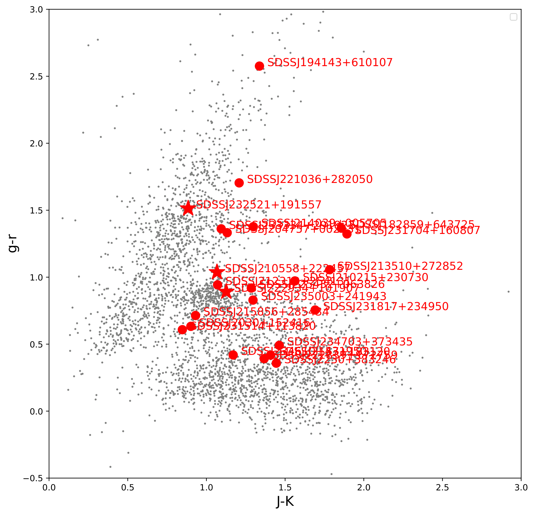
The principal result is empirical mapping of spectroscopic classes across clean and transitional g−r versus J−K regions: the stellar-region target was a star, all four safe-quasar targets were normal quasars, and all ten confirmed quasars in transitional regions were BALs. This supports an association between colour ambiguity and BAL incidence, not a demonstrated causal mechanism. The lowest-z quasar (z=0.139) is only said to be reminiscent of an LRD; no matched LRD spectral, size, or physical-property analysis is reported. [3][1]
Limits and open questions
The sample is small and purposively drawn from selected colour-space regions, so the reported BAL concentration requires a larger systematic sample. AV values rely on simple reddened-template treatment: two BAL spectra have suppressed blue continua not reproduced by the adopted SMC-like template, for which a steeper curve is suggested. Optical spectra also have about 5% second-order contamination beyond 9000 Å, and some displayed SPHEREx spectra are blended with brighter neighbours. [3][5][10]
Assessment is based on supplied abstract, selected HTML passages, and figure captions; tables, detailed fitting procedures, individual-object measurements, and the quantitative basis for AV uncertainties were not supplied.
Key figures
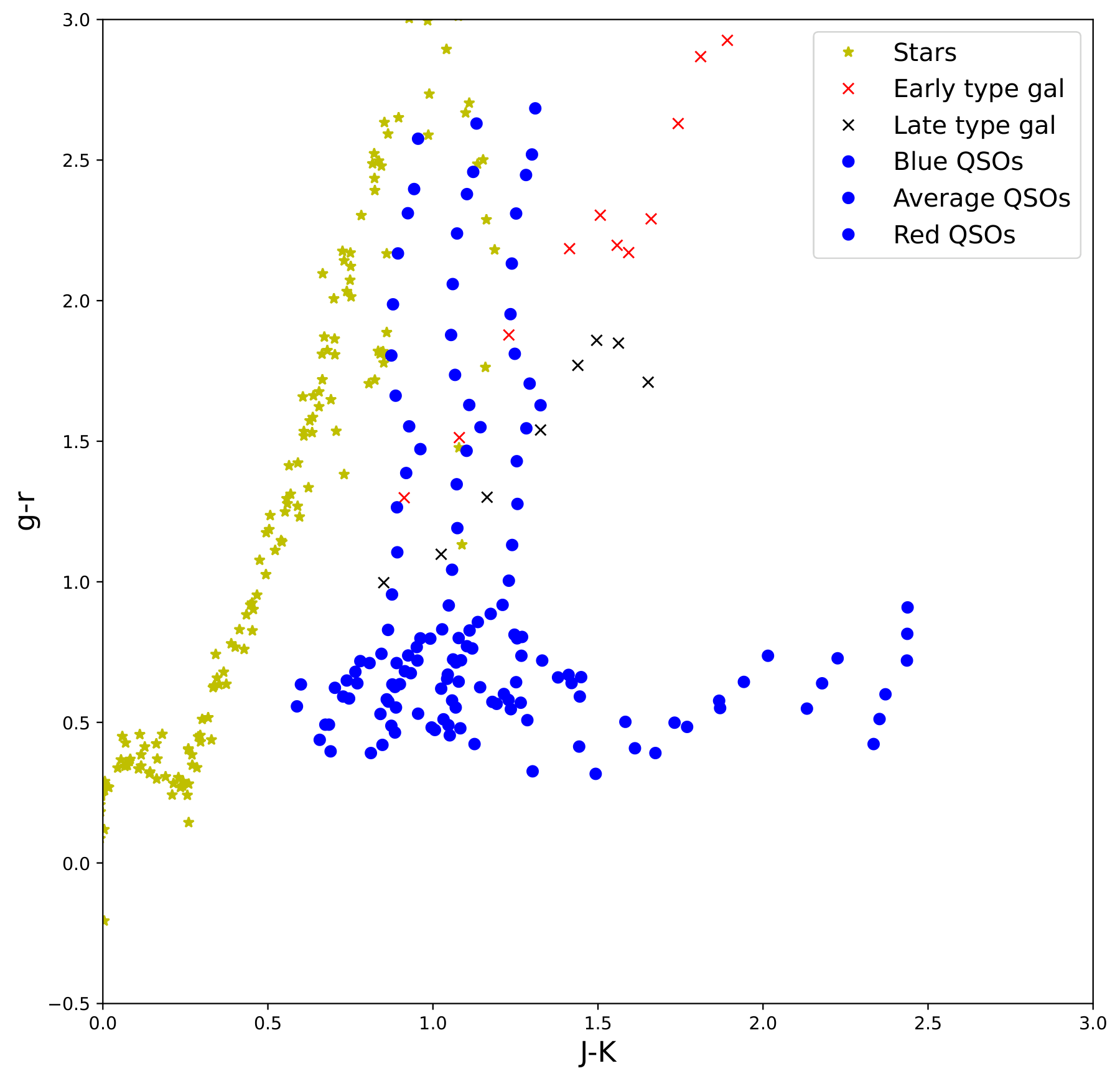
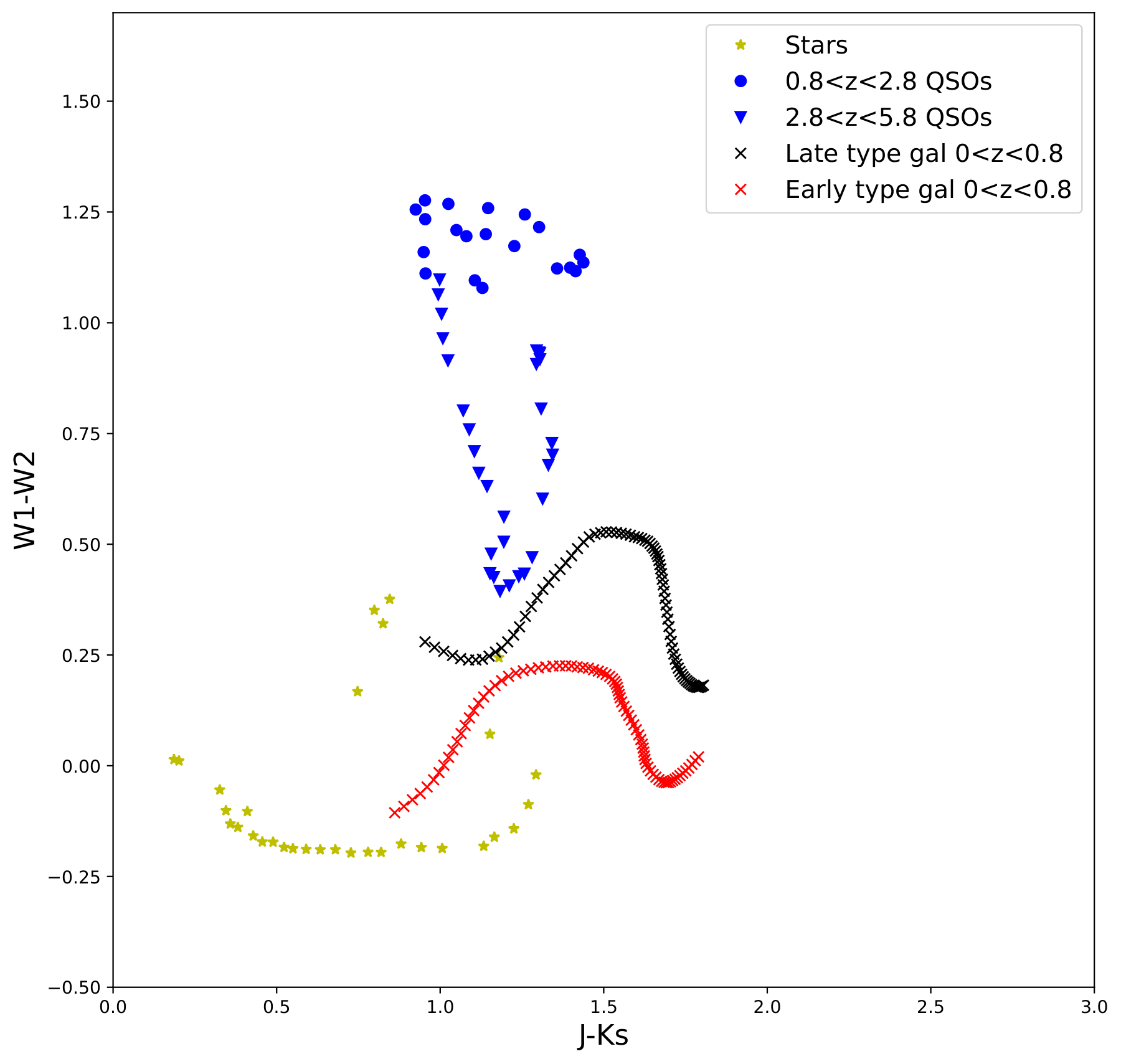
Tests whether theoretical stellar, galaxy, and quasar colour tracks correspond to the observed master catalogue and confirmed-object locations—the basis for defining cleaner versus ambiguous photometric regions.
Original caption
Figure 2: Colour–colour diagrams. Top panels: Theoretical colour-tracks for stars, galaxies and quasars. Top Left: Colours derived using the templates from Hewett et al. (2006) as described in Fynbo et al. (2017) . Top Right: For this diagram we calculate synthetic colours using templates from Assef et al. (2010) ; Husser et al. (2013) ; Selsing et al. (2016) . Bottom panels: colours of objects in the master catalogue. Confirmed quasars are shown with filled circles and stars with an asterisk.
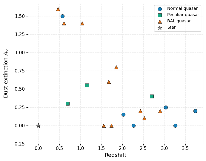
Plots fitted AV against redshift for confirmed quasars, testing the reported tendency for the most extinguished objects to occur mainly at lower redshift rather than establishing a quantitative evolutionary relation.
Original caption
Figure 28: Estimated dust extinction, A V A_{V} , as a function of redshift for the confirmed quasars. Different marker shapes indicate the spectral classifications of the quasars. The most highly extinguished objects are found predominantly at relatively low redshifts.
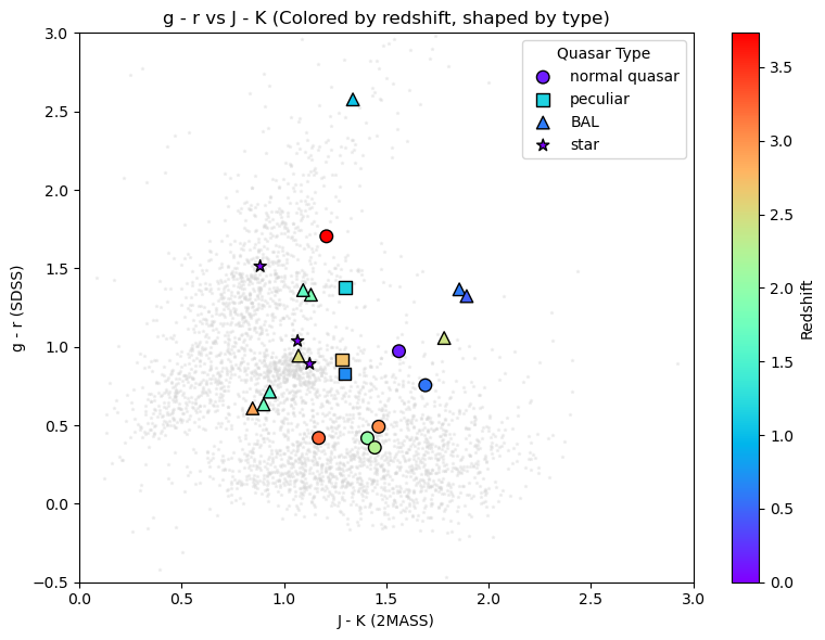
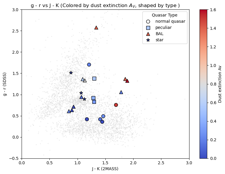
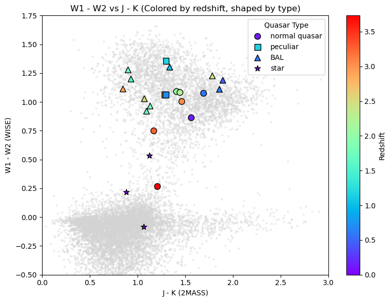
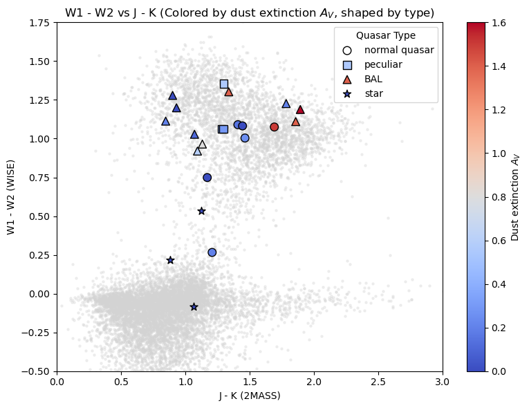
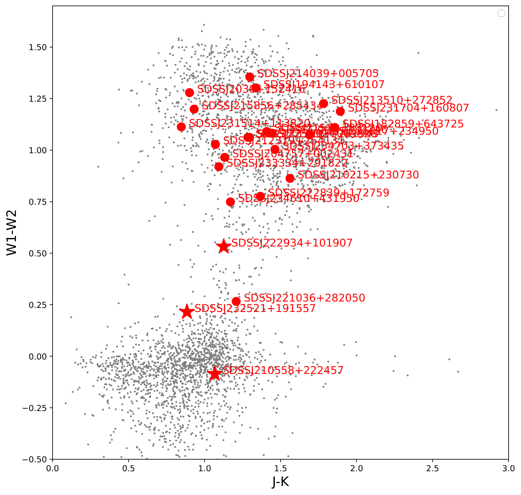
Places spectroscopically observed targets against the full zero-proper-motion population in optical/near-IR and WISE/near-IR colour planes, testing how redshift, fitted extinction, and spectral class populate the selection space.
Original caption
Figure 30: Colour–colour diagrams showing the locations of the spectroscopically observed targets. The top panels show g − r g-r versus J − K J-K , while the bottom panels show W 1 − W 2 W1-W2 versus J − K J-K . Marker shapes indicate the spectroscopic classifications of the targets. In the left panels, quasars are coloured according to their redshifts, while in the right panels they are coloured according to their estimated dust extinctions, A V A_{V} . Grey background points represent objects in the full zero-proper-motion sample. Stars are shown using a fixed colour, since redshift and quasar extinction estimates are not applicable to them.
Related research
Previous digest
Cheng et al. test a deliberately non-complete quasar-selection strategy that first requires Gaia EDR3 sources to have parallax and proper motion consistent with zero, then samples their positions across SDSS, 2MASS, and WISE colour-colour space for spectroscopy. Among 24 observed candidates, they identify 21 quasars spanning z=0.139–3.732 and three stars, with objects displaced from the normal quasar colour locus predominantly turning out to be broad-absorption-line quasars, including FeLoBAL systems. The lowest-redshift quasar, SDSS J210215+230730 at z=0.139, has an LRD-like spectral appearance, illustrating how astrometric pre-selection can uncover unusual reddened or outflow-dominated quasars that colour-only searches can underrepresent.
Sources and evidence (26)
- 2610.19838v1: A heterogeneous set of unusual quasars selected from astrometry and broad-band photometry
The aim of this study is to explore methods for how to identify new quasars with different properties with regard to reddening, redshift, the presence of broad absorption lines from outflows, or other rare properties affecting the broad-band colours. We use Gaia-based astrometric pre-selection to study only sources that have zero parallax and zero proper motion within errors. We subsequently match these sources with information from wide-area photometric surveys and build colour-colour diagrams. Based on these diagrams we select targets for follow-up spectroscopy. In the subsequent analysis we also apply observations from SPHEREx to firmly establish redshifts. We secure spectroscopic observations for 24 sources. Of these, three are found to be stars and the remaining 21 are classified as quasars spanning a redshift range from z=0.139 to z=3.732. The majority of the sources located away from the normal quasar locus in colour-colour diagrams are found to be broad-absorption-line quasars. A single source, the lowest redshift source at z=0.139, is reminiscent of the so-called Little Red Dots found at high redshifts with JWST. Using the simple procedure followed here it is possible to locate previously undiscovered quasars with interesting properties, in particular Broad Absorption Line quasars and quasars with unusual extinction.
- 2610.19838v1: A heterogeneous set of unusual quasars selected from astrometry and broad-band photometry
We investigated 24 quasar candidates selected using Gaia astrometry and multi-wavelength photometry, with targets sampled from both relatively clean and transitional regions of the g − r g-r versus J − K J-K colour–colour diagram. Spectroscopic observations confirm 21 quasars and three stars. The quasars span z = 0.139 z=0.139 – 3.732 3.732 and have estimated extinction values of A V = 0 A_{V}=0 – 1.7 1.7 . Seven are classified as normal quasars (one of which is reminiscent of an LRD), 11 as BAL quasars, and three as peculiar quasars with weak emission lines.
- 2610.19838v1: A heterogeneous set of unusual quasars selected from astrometry and broad-band photometry
The classifications in the relatively clean regions agree with the theoretical expectations: the single target selected from the stellar region was confirmed as a star, while all four targets selected from the safe quasar region were confirmed as normal quasars. In contrast, the transitional regions contain both stars and quasars, and all ten quasars confirmed there are BAL quasars. This suggests that BAL quasars may occur more frequently in photometrically ambiguous regions, although a larger and more systematic sample is required to test this possibility.
- 2610.19838v1: A heterogeneous set of unusual quasars selected from astrometry and broad-band photometry
The addition of near-infrared spectra from SPHEREx was particularly useful in confirming redshifts when optical spectra were complex or difficult to interpret, including SDSS J182859+643725, SDSS J194143+610107, SDSS J212319+254131 and SDSS J214039+005705.
- 2610.19838v1: A heterogeneous set of unusual quasars selected from astrometry and broad-band photometry
Two BAL quasars also show unusually suppressed blue continua that cannot be reproduced well by the adopted SMC-like reddened template. A steeper extinction curve may provide a possible explanation.
- 2610.19838v1: A heterogeneous set of unusual quasars selected from astrometry and broad-band photometry
Overall, our results show that combining astrometric selection, colour–colour sampling, and optical and near-infrared spectroscopy is effective for identifying quasars with unusual absorption and reddening properties.
- 2610.19838v1: A heterogeneous set of unusual quasars selected from astrometry and broad-band photometry
Starting this year, the Purely Astrometric Quasar Survey ( Krogager et al., 2023 , PAQS,) will start building up a sample of of order 300.000 sources selected from Gaia astrometry down to a Gaia G G magnitude limit of 20.5 and followed up spectroscopically with the 4MOST instrument in Chile. This survey will sample the whole colour space (including the position of the stellar track) and will hopefully give us a clean census of the quasar population down to the survey flux limit.
- 2610.19838v1: A heterogeneous set of unusual quasars selected from astrometry and broad-band photometry
The paper is organized in the following way: In Sect. 2 we describe how the targets of this study have been selected. In Sect. 3 we describe the observations, which mostly come from a summer school in August 2024, with additional observations extending the sample in 2025. In Sect. 4 we describe our results, which mainly consists of analysis of the spectra and classification of the sources in terms of object class (star or quasar, which type of quasar), extinction and redshift. In Sect. 5 we discuss the implications of our work and in Sect. 6 we provide our conclusions.
- 2610.19838v1: A heterogeneous set of unusual quasars selected from astrometry and broad-band photometry
These results show that the theoretical tracks provide a useful first-order description of the source distribution, while the mid-infrared information offers an independent but imperfect empirical discriminator. Their combination identifies regions in which photometric classification is relatively reliable, as well as regions in which spectroscopic follow-up remains essential.
- 2610.19838v1: A heterogeneous set of unusual quasars selected from astrometry and broad-band photometry
Most targets were observed using grism 4, which provides a wavelength coverage of approximately 3200–9600 Å with a spectral resolution of slightly below 400 when using a 1” slit. This setup is well suited for identifying prominent emission and absorption features in quasar spectra over a wide redshift range. A subset of targets was re-observed using grism 20, covering the wavelength range 5650–10150 Å, to obtain follow-up spectra with improved sensitivity at longer wavelengths and approximately double the resolution compared to grism 4. Both grism 4 and grism 20 suffer from about 5% 2nd-order contamination redward of 9000 Å. This combination of grisms offers broad wavelength coverage while maintaining a suitable balance between spectral resolution and signal-to-noise ratio for reliable spectral classification and redshift determination. A complete list of the observed targets, together with their coordinates and observational parameters, is provided in Table 1 and Table 2 .
- 2509.07611v1: Balmer Absorption in Iron Low-Ionization Broad Absorption Line Quasars
§ II describes the sample and extraction of the spectra. § III discusses the spectral fitting and extraction of parameters. § IV includes the correlation analysis. § V discusses what we can learn about the physical properties of FeLoBAL quasar absorption from the results, and it also compares FeLoBAL quasar properties with those of LRDs. It turns out that there are similarities in the emission lines and in the spectral energy distribution, including the lack of hot dust emission, the extreme reddening and blue emission, and lack of X-ray emission. § VI summarizes the results. Throughout we use typical cosmological parameters (H 0 = 69.32 km Mpc − 1 s − 1 {}_{0}=69.32\rm\,km\,Mpc^{-1}\,s^{-1} , Ω c = 0.233 \Omega_{c}=0.233 , Ω Λ = 0.721 \Omega_{\Lambda}=0.721 ).
- 2509.07611v1: Balmer Absorption in Iron Low-Ionization Broad Absorption Line Quasars
Table 2: Spectral Fitting Results
- 2607.27329v1: An Exploratory Analysis of New Large Gaia-informed Quasar Samples in SDSS-V
The quasar selection methods that produced our sample(s), which were based on previous works by 113 and 127 , have proven to be powerful ways to produce a large, highly efficient, all-sky quasar sample. The quasar selection efficiency of GUA, which relies solely on Gaia and unWISE data, exceeded 96%, and remains high even at low Galactic latitudes (see Section IV.2 and Figure 9 ).
- 2607.27329v1: An Exploratory Analysis of New Large Gaia-informed Quasar Samples in SDSS-V
While the photometric properties of the bulk of the GUA and Skewt_QSO samples are broadly consistent with those of previous quasars catalogs (e.g., SDSS/DR7Q), they do cover a wider range in optical and/or IR color spaces, which allows to probe larger populations of red, mildly-obscured AGNs (see Section IV.3 ). A significant fraction ( ≈ 26 % {\approx}26\% ) of our quasars satisfies the R − W 1 > 4 R-W1>4 obscuration criterion of LaMassa et al. [65] , intermediate between samples based on optical color selection (i.e., DR7Q quasars) and on X-rays (i.e., LaMassa et al. 66 ; see Fig. 13 ). So far the GUA and Skewt_QSO programs have not identified extremely obscured systems, such as Hot DOGs (mainly due to flux limits; see Fig. 14 ).
- 2607.22835v1: Unsupervised selection and characterisation of Little Red Dots in JWST surveys with manifold learning
A central point for interpreting our results is that the parent sample is itself the product of a selection function, and we quantify its effect on the spectroscopic LRDs explicitly. Of the 116 unique spectroscopically selected LRDs of de Graaff et al. (2025) , 89 ( 77 % 77\% ) fall within the footprint and detection limits of our parent catalogue. Of these, 68 ( 59 % 59\% of the original 116) additionally satisfy the pre-processing requirements above and enter the final sample. The losses are not random in redshift: the sources removed by pre-processing have a higher median redshift ( z ≃ 5.6 z\simeq 5.6 ) than those retained ( z ≃ 5.1 z\simeq 5.1 ). Waiving the detection requirement in F814W, i.e., allowing it to be undetected (Section 2.3 ), already recovers the most common dropout cases, but a detection is still required in the bluer NIRCam bands, so the very reddest and highest-redshift sources (faint or absent in F115W and F150W) continue to be preferentially removed; this residual imprint of the detection requirement on the high-redshift tail is the dominant bias of the parent selection.
- 2607.22835v1: Unsupervised selection and characterisation of Little Red Dots in JWST surveys with manifold learning
The structure is intrinsic, not a projection artefact (Section 4.2 ). The same localisation is present in the original feature space, and a cross-validated classifier recovers ∼ \sim 90% of held-out spectroscopic LRDs, confirming that the location generalises.
- 2604.13178v1: 4MOST ChANGES: Catalog of high-redshift quasar candidates (4.5 < $z$ < 7) selected with SED fitting
With this approach, we reach 44% completeness and 1.5% reliability (see Figure 9 ). Here, reliability is computed as the fraction of our selected candidates that are spectroscopically confirmed quasars from the F23 sample; the remaining candidates have not been spectroscopically confirmed and should not be assumed to be contaminants. The pink points in the top panel of Figure 9 represent our unconfirmed quasar candidates. Therefore, given the incompleteness of southern sky spectroscopic samples, the measured reliability should be interpreted as a conservative lower limit rather than a definitive estimation of our selection’s true performance. A full assessment of completeness and reliability would require modeling the selection function to quantify the impact of each selection criterion, which is deferred to future work after dedicated spectroscopic follow-up.
- 2604.13178v1: 4MOST ChANGES: Catalog of high-redshift quasar candidates (4.5 < $z$ < 7) selected with SED fitting
dshift quasars (see Figure 10 ). The third target (Object ID 10735100050971)is likely an M-type star (see Table 2 ). Overall, our spectroscopic campaign achieved a detection rate of 50% (3 confirmed quasars out of 6 observed candidates). However, we note that this rate is not representative of the full catalog, as these candidates were specifically selected based on their brightness and visual inspection. The true reliability of our selection will be determined once spectroscopic information is obtained for the entire catalog. It is important to note that all these sources were selected from our catalog of high-redshift quasar candidates based on their z z -band magnitudes ( z m a g , d e c a l s < 20.5 z_{mag,decals}<20.5 ). We also visually inspected their images in the Legacy Survey Sky Viewer and PanSTARRS-1 Image Access to prioritize bright and clear point-like sources.
- 2512.02096v1: Discovery of two little red dots transitioning into quasars
Figure 2 : JWST NIRCam F444W slitless spectra of the Forges . We also show the best-fit results and associated residuals. Prominent emission features (e.g., He i , O i λ 11287 \lambda 11287 , Pa γ \gamma , Pa δ \delta ) are labeled. Short vertical lines at the top, labeled with line names, mark the theoretical positions of the emission lines. For Forge II , A zoom-in on the Pa δ \delta absorption feature is shown in the subpanel, and additional spectroscopic coverage from DESI (covering the wavelength ranges of Ly α \alpha , N v , O i λ 1304 \lambda 1304 , C iv , He ii , and C iii] ) and HST G141 (Mg ii ) is also displayed. The gray-shaded regions indicate the wavelength ranges masked during the fitting process due to contamination from neighboring sources in the NIRCam spectra.
- 2512.02096v1: Discovery of two little red dots transitioning into quasars
We estimate the central BH masses M BH M_{\mathrm{BH}} and bolometric luminosities L bol L_{\rm bol} of the Forges using the spectral and photometric data above. We first model their continuum and line emission and absorption features in the JWST slitless spectra (Methods), and the best-fit results are listed in Extended Data Table 1 . The full widths at half maximum (FWHM) of the emission lines are about several thousand km s -1 , confirming their AGN nature. In addition, the strong O i λ 11287 \lambda 11287 emission agrees with the predicted signature of high-accretion SMBHs 29 . Assuming that these lines originate from the AGN broad-line regions, we calculate BH mass using the broad Paschen emission lines and the 1 μ \mu m continuum luminosity 30 . The resultant masses are ( 3.72 ± 1.86 ) × 10 8 M ⊙ (3.72\pm 1.86)\times 10^{8}\,M_{\odot} and ( 9.78 ± 4.89 ) × 10 8 M ⊙ (9.78\pm 4.89)\times 10^{8}\,M_{\odot} ( M ⊙ M_{\odot} is the Solar mass), respectively. Forge II was also observed by the DESI spectroscopic survey and HST G141 slitless spectroscopy. Only narrow Ly α \alpha emission line (FWHM = 556 km s − 1 =556\rm\penalty\ km\penalty\ \,s^{-1} ) is detected by DESI, shown in the lower panel of Figure 2 . Canonical AGN broad lines, including Ly α \alpha , N v λ 1240 \lambda 1240 , C iv λ 1549 \lambda 1549 , He ii λ 1640 \lambda 1640 , and C iii] λ 1909 \lambda 1909 , are not detected, which is consistent with previous results that high-redshift LRDs have weak or no broad UV emission lines 7 , 28 . We assume that the central AGNs are obscured in the rest-frame UV, but dominate in the near-IR, radio, and X-ray bands, then we obtain AGN bolometric luminosities L bol L_{\rm bol} by integrating their reprocessed SEDs (Extended Data Figure 3 ). The inferred Eddington ratios are L bol / L Edd = 0.17 − 0.08 + 0.25 L_{\rm bol}/L_{\rm Edd}=0.17^{+0.25}_{-0.08} and 0.24 − 0.12 + 0.42 0.24^{+0.42}_{-0.12} , where the Eddington luminosity is L Edd = 1.3 × 10 38 ( M BH / M ⊙ ) erg s − 1 L_{\rm{Edd}}=1.3\times 10^{38}\ (M_{\rm{BH}}/M_{\odot})\ \rm{erg\ s^{-1}} .
- 2512.18421v1: The evolution of obscured AGN across cosmic time -- A large quasar survey for the 2040s
In addition, Vera C. Rubin Observatory’s Legacy Survey of Space and Time (LSST) will provide millions of candidates via intrinsic variability; a method less sensitive to obscuration. Dedicated spectroscopic monitoring of these candidates will uncover hundreds of thousands of CL AGN and probe the intrinsic accretion disk and Broad Line Region (BLR) in heavily reddened systems. This offers a new method to disentangle between orientation, evolutionary stage, and accretion state changes in obscured versus unobscured systems. Using multi-epoch spectroscopy to track obscuration changes, BLR re-emergence, and disk- wind signatures over time will provide unique, direct constraints on the physical origin and evolution of obscuration. While identifying 50 million quasars yields an exceptionally large sample, such volume is essential to correct for selection biases. For instance, FeLoBALs were originally thought to be extremely rare based on the SDSS survey (>100,000 quasars), representing less than 1% of the population (Trump et al. 2006). However, radio and mid-infrared selection revealed the fraction to be significantly higher (~10%; Urrutia et al. 2009; Dai et al. 2012). To achieve completeness and ensure a statistically representative sample of at least 100 objects per class, luminosity, and redshift bin, a dataset of this magnitude is required. 4. Necessary technology developments While current large MOS instruments capable of 1000–5000 simultaneous spectra are mounted on 2–4m class telescopes, the next generation of surveys demands significantly greater capability. Current facilities being developed for the ELT can observe only a relatively small number of targets in very deep fields. Characterizing over 50 million AGN targets, particularly at faint magnitudes and high redshifts, requires a facility combining high multiplexing (20,000–30,000 spectra) with a 10–15m aperture, such as the Wide-Field Spectroscopic Telescope (WST, Mainieri et al. 2024). This increased collecting area is critical for obtaining spectra of heavily obscured sources (NH ~ 1024 cm-2), reaching down to 25th magnitude with low-medium spectral resolution (R~1500) and achieving a S/N > 5 in the po
- 2512.18421v1: The evolution of obscured AGN across cosmic time -- A large quasar survey for the 2040s
The evolution of obscured AGN across cosmic time A large quasar demographic optical MOS survey targeting over 50 million AGN candidates Tanya Urrutia1, Darshan Kakkad2, Paula Sánchez-Sáez3, Mojtaba Raouf4,5, Swayamtrupta Panda6, Sarah E I Bosman7, Francisco Pozo Nunez8, Annagrazia Puglisi9, Sophia Flury10, Dragana Ilic11, Andjelka B. Kovacevic11, Mamta Pandey- Pommier12, Giustina Vietri13, Sarath Satheesh-Sheeba14, Francesco Salvestrini15, Susanna Bisogni13, Eduardo Bañados16, Ana Monreal Ibero4, Sabine Thater17, Pratika Dayal18, Filippo D’Ammando19, José Afonso20, Paramita Barai15, Valentin Ivanov3 [1] Leibniz-Institut für Astrophysik, Potsdam (AIP), An der Sternwarte 16, 14482, Potsdam, Germany [2] Centre for Astrophysics Research, Department of Physics, Astronomy and Mathematics, University of Hertfordshire, Hatfield, AL10 9AB, UK [3] European Southern Observatory, Karl-Schwarzschild-Str. 2, 85748 Garching bei München, Germany [4] Leiden Observatory, Leiden University, P.O. Box 9513, 2300 RA Leiden, Netherlands [5] Faculty of Aerospace Engineering, Delft University of Technology, Delft, The Netherlands [6] International Gemini Observatory, NSF NOIRLab, Casilla 603, La Serena, Chile [7] Institute for Theoretical Physics, University of Heidelberg, Philosophenweg 12, Heidelberg 69115, Germany [8] Heidelberg Institute for Theoretical Studies, Astroinformatics, Schloss-Wolfsbrunnenweg 35, 69118 Heidelberg, Germany [9] School of Physics and Astronomy, University of Southampton, Highfield, SO17 1BJ, UK [10] Institute for Astronomy, Royal Observatory, University of Edinburgh, Edinburgh EH9 3HJ [11] University of Belgrade, Faculty of Mathematics, Studentski trg 16, 11000 Belgrade, Serbia [12] Pole Scientific, University Catholic of Lyon- University of Lyon, 10 place des Archives 69288, Lyon, France [13] INAF IASF-Milano, Istituto di Astrofisica Spaziale e Fisica cosmica Milano, Via Alfonso Corti 12 20133 [14] Instituto de Astrofísica, Facultad de Ciencias Exactas, Universidad Andres Bello, Fernández Concha 700, 7591538 Las Condes, Santiago, Chile [15] INAF Osservatorio Astronomico di Trieste, via G.B. Tiepolo 11, 34143 Trieste, Italy [16] Max-Planck-Insititute für Ast
- 2601.08936v1: A possible pathway to UHZ1-type systems at z~10 by heterogeneous mass primordial black holes as dark matter
We can now tie this discussion to Fig. 2 which indicates the halo mass range that can collapse at any z z , for various f PBH M PBH f_{\rm PBH}M_{\rm PBH} and ( 1 , 3 ) σ (1,3)\sigma density excursions. The figure shows that at the 3 σ \sigma level, halos of M H ≃ ( 1.5 × 10 5 , 3 × 10 5 , 7 × 10 5 , 2.5 × 10 6 , 10 7 ) M ⊙ M_{\rm H}\simeq(1.5\times 10^{5},3\times 10^{5},7\times 10^{5},2.5\times 10^{6},10^{7})M_{\odot} , can collapse at z = 100 , 70 , 50 , 30 , 20 z=100,70,50,30,20 , if f PBH M PBH = 20 M ⊙ f_{\rm PBH}M_{\rm PBH}=20M_{\odot} , decreasing to M H ≃ ( ≤ 10 5 , 1.7 × 10 5 , 4 × 10 5 , 1.3 × 10 6 , 5 × 10 6 ) M ⊙ M_{\rm H}\simeq(\leq 10^{5},1.7\times 10^{5},4\times 10^{5},1.3\times 10^{6},5\times 10^{6})M_{\odot} at z = 100 , 70 , 50 , 30 , 20 z=100,70,50,30,20 , if f PBH M PBH = 10 M ⊙ f_{\rm PBH}M_{\rm PBH}=10M_{\odot} . The Press-Schechter ( 66 ) formalism suggests that a sufficient fraction of such halos would exist at ( 3 − 5 ) σ (3-5)\sigma levels to produce - for suitable PBH mass functions - at least a few central objects of 10 7 − 10 8 M ⊙ 10^{7}-10^{8}M_{\odot} by z = 10 z=10 , as observed for UHZ1. E.g., at 3 σ 3\sigma we can expect ≃ 0.3 % \simeq 0.3\% of the density field to have the required parameters. Currently, theoretically-motivated PBH mass function proposals contain 10 to 20% by mass in PBHs of 10 M ⊙ 10M_{\odot} or higher ( 12 ) , i.e., those subject to dynamical friction, and 10-20% of them will have the required low angular momentum, λ ≤ 0.1 − 0.2 \lambda\leq 0.1-0.2 . Dynamical friction would therefore drive ∼ 1 − 2 % \sim 1-2\% of the total mass of the PBH component to the central 1 pc in ( 0.5 − 1 ) × t cosm (0.5-1)\times t_{\rm cosm} after halo collapse. These clusters of PBHs at the centers of low mass halos will merge into larger units as hierarchical clustering proceeds. At z ≃ 15 z\simeq 15 , halos of 10 9 M ⊙ 10^{9}M_{\odot} , corresponding to peaks of 3 − 4 σ 3-4\sigma , could have collapsed and given rise to concentrations of up to ∼ 10 7 M ⊙ \sim 10^{7}M_{\odot} in the central parsec by z = 10 z=10 , depending on the fraction, f PBH f_{\rm PBH} , of DM consisting of PBHs. Baryonic accret
- 2601.08936v1: A possible pathway to UHZ1-type systems at z~10 by heterogeneous mass primordial black holes as dark matter
Figure 3: Dynamical friction collapse time t df t_{\rm df} from solving numerically eqs. 6 , in units of the crossing/orbital time, R H / V 0 R_{\rm H}/V_{0} as a function of λ \lambda and 𝒞 {\cal C} . These results correspond to m ∙ ln Λ / M H = 0.01 m_{\bullet}\ln\Lambda/M_{\rm H}=0.01 and can be rescaled to other values since t df ∝ ( m ∙ ln Λ / M H ) − 1 t_{\rm df}\propto(m_{\bullet}\ln\Lambda/M_{\rm H})^{-1} . Dashed horizontal lines mark ( 1 , 2 , 3 ) × t cosm ( z ) (1,2,3)\times t_{\rm cosm}(z) , whereas the dotted line indicates the time for an individual halo to remain intact from z = 50 z=50 to z = 10 z=10 . Left: t df t_{\rm df} vs. λ \lambda ; NFW halo profiles with 𝒞 = 10 , 20 , 30 , 40 , 100 {\cal C}=10,20,30,40,100 , are shown with blue, orange, green, red, and purple solid lines, and isothermal halo profiles with the same concentrations are shown with corresponding dash-dotted lines. The isothermal, non-truncated distribution ℱ ( E ) {\cal F}(E) was adopted. Right: Same vertical axis vs. the concentration parameter, 𝒞 {\cal C} . Solid lines represent NFW profiles with λ = 0.05 , 0.1 , .0.15 , 0.2 , 0.3 \lambda=0.05,0.1,.0.15,0.2,0.3 in blue, orange, green, red, and purple, respectively, and dash-dotted lines correspond to isothermal profiles.
- 2501.09585v1: New Methods of Identifying AGN in the Early Universe using Spectroscopy and Photometry in the JWST Era
In conclusion, although this photometry analysis cannot be used as a completely independent diagnostic tool for finding AGN in galaxies, it can still be a good resource to accompany spectroscopic analysis. By looking first at the spectroscopy of the galaxies that pass our criteria, we can prioritize the galaxies that have a higher probability of being an AGN. Nonetheless, we should not claim that a galaxy is not an AGN just by the results of the photometric analysis, but would need further confirmation from spectroscopy to back up the finding of AGN in these systems.
- 2501.09585v1: New Methods of Identifying AGN in the Early Universe using Spectroscopy and Photometry in the JWST Era
In this paper we explore how to identify active galactic nuclei (AGN) within galaxies with data from the JWST. We show that existing optical diagrams such as the BPT diagram and the VO87 diagram pose limitations when analysing AGN at high redshifts. These limitations include significant regions where AGN and SFG overlap, and missing lines outside the JWST’s detection range, rendering analysis impossible. Therefore, new methods and ideas are needed to make progress within this very important topic.
Abstract
The aim of this study is to explore methods for how to identify new quasars with different properties with regard to reddening, redshift, the presence of broad absorption lines from outflows, or other rare properties affecting the broad-band colours. We use Gaia-based astrometric pre-selection to study only sources that have zero parallax and zero proper motion within errors. We subsequently match these sources with information from wide-area photometric surveys and build colour-colour diagrams. Based on these diagrams we select targets for follow-up spectroscopy. In the subsequent analysis we also apply observations from SPHEREx to firmly establish redshifts. We secure spectroscopic observations for 24 sources. Of these, three are found to be stars and the remaining 21 are classified as quasars spanning a redshift range from z=0.139 to z=3.732. The majority of the sources located away from the normal quasar locus in colour-colour diagrams are found to be broad-absorption-line quasars. A single source, the lowest redshift source at z=0.139, is reminiscent of the so-called Little Red Dots found at high redshifts with JWST. Using the simple procedure followed here it is possible to locate previously undiscovered quasars with interesting properties, in particular Broad Absorption Line quasars and quasars with unusual extinction.
Discussion
Discussion access requires a security token. Register for the weekly digest.